How to Filter Google Sheets: Quick and Easy Steps for Data Organization

Google Sheets is a powerful tool for organizing and analyzing data. One of its most useful features is the ability to filter information quickly and easily. You can filter in Google Sheets by using the built-in filter feature or the FILTER function.

The built-in filter lets you sort and hide data without changing your original spreadsheet. It’s great for temporary views of your data. The FILTER function, on the other hand, lets you create new datasets based on specific conditions you set.

Whether you’re managing a large inventory, tracking sales data, or organizing personal information, learning to filter in Google Sheets can save you time and make your data more manageable. In this guide, we’ll walk you through both methods step-by-step.

Understanding Filters in Google Sheets

Filters in Google Sheets let you sort and view specific data. They help you find what you need quickly and easily. You can use different types of filters to organize your information.

Fundamentals of Filtering

Filters in Google Sheets are tools that help you see only the data you want. To use a filter, click on the filter icon at the top of a column. This adds a dropdown menu to your column headers.

You can filter by:

• Text
• Numbers
• Dates
• Colors

When you apply a filter, it hides rows that don’t match your criteria. This doesn’t delete any data. It just changes what you see on screen.

You can use multiple filters at once. This lets you narrow down your data even more.

Types of Filters

Google Sheets offers several ways to filter your data:

1. Value Filters: These let you pick specific values to show or hide.
   
2. Condition Filters: You can set rules like “greater than” or “contains” to filter data.
   
3. Color Filters: These filter cells based on their background or text color.
   
4. Formula Filters: You can use the FILTER function to create more complex filters.
   

Each type of filter serves a different purpose. Choose the one that fits your needs best.

Filter Views vs Regular Filters

Filter Views and Regular Filters are two ways to filter data in Google Sheets.

Regular Filters:

• Apply to everyone viewing the sheet
• Change the view for all users
• Are good for permanent changes

Filter Views:

• Only affect your view of the sheet
• Don’t change what others see
• Let you save different filter setups

Filter Views are great when you want to analyze data without affecting others. Regular Filters work well for shared data that everyone needs to see the same way.

Choose Filter Views when you need personal data views. Use Regular Filters for consistent team views.

Working with the Filter Function

The Filter function in Google Sheets helps you sort data easily. It lets you pick out specific information from a big set of data.

Syntax of the Filter Function

The Filter function in Google Sheets uses this basic form:

=FILTER(range, condition1, [condition2, …])

“Range” is the data you want to filter. “Condition1” is the first rule you set. You can add more rules if needed.

Here’s a simple example:

=FILTER(A2, A2>5)

This formula picks rows where column A has numbers bigger than 5.

You can use other functions inside FILTER. For instance:

=FILTER(A2, ISTEXT(B2))

This picks rows where column B has text.

Filter Function Best Practices

When using the FILTER function, keep these tips in mind:

1. Check your data range: Make sure it’s right before you filter.
2. Use clear conditions: Simple rules work best.
3. Test your formula: Try it on a small set of data first.

For complex filters, you can combine conditions:

=FILTER(A2, A2>5, B2=”Yes”)

This picks rows where A is more than 5 and B is “Yes”.

Be careful with blank cells. They can mess up your results. Use ISBLANK() to deal with them:

=FILTER(A2, NOT(ISBLANK(A2)))

This removes rows where column A is empty.

Applying Simple Filters

Filters in Google Sheets let you quickly sort and analyze your data. You can use them to show only the information you need.

Filter by Single Condition

To filter by a single condition, click the filter icon at the top of a column. Choose “Filter by condition” from the menu. You’ll see options like “Text contains” or “Greater than” for numbers.

Pick the rule that fits your needs. For example, to find names starting with “A”, select “Text starts with” and type “A”.

Click “OK” to apply the filter. Your sheet will now show only the rows that match your condition.

You can add more rules to narrow down your results. Just click “Add another condition” in the filter menu.

Sorting and Filtering by Values

Filtering by values lets you choose specific items to show or hide. Click the filter icon and select “Filter by values”.

You’ll see a list of all unique values in that column. Uncheck the boxes next to items you want to hide.

For sorting, use the “Sort A to Z” or “Sort Z to A” options in the filter menu. This arranges your data in alphabetical or numerical order.

You can also filter by color if you’ve used cell colors to organize your data. This is helpful for visual sorting.

Remember, you can always clear a filter by clicking the filter icon and selecting “Clear filter”.

Advanced Filtering Techniques

Google Sheets offers powerful tools to refine your data analysis. These methods let you sift through complex datasets with precision and ease.

Using Multiple Conditions

You can filter data using multiple criteria in Google Sheets. This helps narrow down results based on specific needs.

To apply multiple filters:

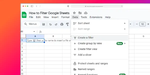
1. Select your data range
2. Click “Data” > “Create a filter”
3. Use the filter buttons in column headers
4. Choose your first condition
5. Click “Add another condition”
6. Select your second condition

You can add more conditions as needed. This method works well for finding data that meets several requirements at once.

Filter by Color and Formatting

Google Sheets allows filtering based on cell colors and formats. This visual approach can quickly sort data you’ve highlighted.

To filter by color:

1. Apply colors to cells you want to filter
2. Click the filter button in the column header
3. Choose “Filter by color”
4. Select the color you want to filter by

This technique helps when you’ve used colors to mark important data or categories. It’s a quick way to find visually tagged information.

Incorporating And/Or Conditions

Advanced filters in Google Sheets can use AND/OR logic for complex sorting. This lets you create very specific data views.

To use AND/OR conditions:

1. Go to “Data” > “Filter views” > “Create new filter view”
2. Click “Add a filter”
3. Choose your first condition
4. Click “Add another condition”
5. Select AND or OR
6. Add your second condition

AND finds data meeting all conditions. OR finds data meeting any condition. You can mix these for detailed filtering.

Dynamic Arrays and Conditional Filtering

Google Sheets offers powerful tools for filtering and organizing data. Dynamic arrays and conditional filters can help you find exactly what you need in large datasets.

Leveraging Dynamic Arrays

Dynamic arrays in Google Sheets automatically expand to include new data. You can use them with the FILTER function to create flexible, updating lists.

To set up a dynamic array filter:

1. Select your data range
2. Use the FILTER formula
3. Add your conditions

For example:

=FILTER(A2:D100, B2:B100="Apples")

This will show all rows where column B contains “Apples”. The array will grow or shrink as you add or remove data.

You can also combine multiple conditions:

=FILTER(A2:D100, B2:B100="Apples", C2:C100>5)

This filters for “Apples” in column B and values greater than 5 in column C.

Filtering with Date Functions

Date functions let you filter data based on time periods. You can use them to find recent entries or compare dates.

To filter by date:

1. Use the DATE function in your FILTER formula
2. Compare it to your date column

Example:

=FILTER(A2:D100, C2:C100>DATE(2024,1,1))

This shows all rows with dates after January 1, 2024 in column C.

You can also use functions like TODAY() for rolling date ranges:

=FILTER(A2:D100, C2:C100>TODAY()-30)

This displays entries from the last 30 days.

Finding Largest Values

To find the largest values in your data:

1. Use the LARGE function
2. Combine it with FILTER for more specific results

For example, to get the top 5 values:

=LARGE(B2:B100, SEQUENCE(5))

You can also filter first, then find the largest:

=LARGE(FILTER(B2:B100, A2:A100="Category A"), SEQUENCE(3))

This finds the 3 largest values in column B where column A is “Category A”.

Remember to adjust your data ranges as needed. These techniques help you quickly analyze and extract key information from your spreadsheets.

Dealing with Complex Data Sets

Filtering complex data in Google Sheets requires specific techniques. These methods help you handle partial matches, empty cells, and custom criteria to get the exact information you need.

Handling Partial Matches

To filter partial matches in Google Sheets, use the Custom filter option. Click the filter icon in the column header and choose “Filter by condition”. Select “Text contains” from the dropdown menu.

Enter the partial text you want to match. This works for names, product codes, or any text data. For example, if you have a list of names and want to find all “John” entries, including “Johnson” or “Johnny”, just type “John”.

You can also use wildcards. The asterisk (*) stands for any number of characters. The question mark (?) replaces a single character. These are helpful for more complex partial matches.

Filtering Out Empty Cells

Empty cells can mess up your data analysis. To filter them out:

1. Click the filter icon in the column header
2. Choose “Filter by condition”
3. Select “Is not empty” from the dropdown

This shows only rows with data in that column. It’s useful for cleaning up spreadsheets or focusing on complete entries.

You can also do the opposite. Select “Is empty” to see which rows are missing data. This helps spot gaps in your dataset that need attention.

Working with Specified Criteria

For more detailed filtering, use specified criteria. This lets you set exact conditions for your data. Here’s how:

1. Click the filter icon
2. Choose “Filter by condition”
3. Pick a condition (like “Greater than” or “Contains”)
4. Enter your criteria

You can combine multiple criteria. Use “Add another condition” to create complex filters. For example, find all sales over $1000 in the month of July.

Custom formulas offer even more control. In the filter menu, select “Custom formula is”. Enter a formula that returns TRUE or FALSE for each row. This method is great for advanced users who need very specific filters.

Best Practices for Filtering Data

Filtering data in Google Sheets can help you find important information quickly. Using the right techniques will make your data easier to work with and understand.

Designing Sustainable Filter Systems

Start by organizing your data in a clear, consistent way. Use headers for each column to make filtering simpler. Think about what filters you’ll use most often and set them up in advance.

Create filter views to save different filter setups. This lets you switch between views without changing the original data. You can save filter views by going to Data > Filter views > Save as filter view.

Use color coding to highlight important data. This makes it easier to spot key information even when filters are applied. Consider freezing the top row so your headers are always visible when scrolling through filtered results.

Avoiding Common Filtering Mistakes

Be careful when using multiple filter conditions. Make sure they work together as intended. For example, using “greater than” and “equal to” at the same time might exclude data you want to see.

Don’t forget to clear filters when you’re done. Leaving filters on can lead to mistakes later. To remove all filters, go to Data > Remove filter.

Check your results after filtering. Make sure the data shown matches what you expected. If something looks off, double-check your filter conditions.

Avoid filtering out blank cells if they contain important information. Instead, use the “Filter by condition” option to include blanks when needed.

Be cautious when editing filtered data. Changes you make might not be visible until you clear the filter. Always review your edits with filters off to ensure accuracy.

Troubleshooting Filter Issues

Is your Google Sheets filter not working as expected? Don’t worry. Many users face this problem. Let’s look at some common issues and how to fix them.

First, check if your filter covers the whole data range. Sometimes, filters only apply to a part of your sheet. To fix this, turn off the current filter and create a new one for the entire sheet.

Make sure your data is consistent. Blank cells or different data types in a column can cause filter problems. Fill in empty cells or remove inconsistent data.

Are you using complex filter conditions? Double-check your filter settings. For “AND” logic, use multiple conditions in one filter. For “OR” logic, create separate filter views.

Try these quick fixes:

• Refresh your browser
• Clear your cache
• Use an incognito window

If nothing works, try removing and recreating your filter. Select your data range, go to “Data” > “Create a filter”.

Remember, filters don’t change your original data. They just hide certain rows. If you need to modify data, use sorting or formulas instead.